02 / Theory

from the chapter, split into four independent parts

Dissolution and diffusion in an evolving porous skeleton

Biodegradation is treated as two coupled local processes: dissolution of the silicon skeleton, and diffusion of the resulting silicic acid through the pore liquid. Everything else on this site — the five morphologies, both limiting solutions, the fitted rate constants — follows from the single system below.

The representative volume

Take a volume ΔV that is large compared with one pore but small compared with the particle. Inside it the local porosity p(r,t) is the pore volume divided by ΔV: p = 0 is solid silicon, p = 1 means the skeleton is gone. The dissolved-silicon concentration is normalised as c = C/C_sat, and because the liquid fills only the fraction p of ΔV, local saturation corresponds to c = p.

This effective-medium picture avoids reconstructing the pore network. The geometry survives in two coefficients only: the effective diffusivity, taken as D_eff(p) = D₀p so the bulk value is recovered as p → 1, and the physical specific surface area S(p), the silicon area inside ΔV divided by ΔV.

Transport and dissolution

Diffusion of dissolved silicon follows Fick’s first law, and the local source is the classical surface-dissolution law of Nernst–Brunner / Noyes–Whitney type:

(1)

(2)

The specific degradation rate k has units of m·s⁻¹, so kS(p) is a volumetric rate coefficient in s⁻¹. The factor (p − c) is what makes dissolution stall as the pore liquid approaches local saturation — the mechanism behind the entire slow-diffusion regime.

Combining the two and imposing conservation of solid silicon gives one coupled system, with ρ_Si the molar density of solid silicon:

(3)

Two geometries

For an isotropic sphere of radius R, symmetry removes the angular dependence and leaves a radial problem with a zero gradient at the centre:

(4, 5)

For a planar layer of thickness L on an impermeable substrate, the flux vanishes at the substrate instead:

(6, 7)

The two formulations differ only in the diffusion operator and the boundary conditions; the local dissolution law is identical.

The world outside the particle

Removal of silicic acid from the outer surface is represented by an external diffusion layer of thickness δ. Matching internal and external fluxes gives a Robin condition, and δ itself follows from the Sherwood number:

(8, 9)

(11)

This is why agitation is the strongest single factor in the measured data: stirring raises Sh, thins δ and keeps the bulk far from saturation. The limiting solutions below use the perfect-sink approximation instead — c_out ≈ 0 and δ → 0, hence c_s ≈ 0.

Which regime are you in?

The competition between dissolution and internal diffusion is measured by a Thiele modulus, equivalently a Damköhler number: the ratio of the diffusion time τ_diff = R²/D_eff to the dissolution time τ_diss = 1/kS(p).

(13)

φ² << 1 is fast internal diffusion; φ² >> 1 is slow internal diffusion. Near unity neither reduction is trustworthy and the full system must be solved numerically — exactly the warning the design calculator raises when your parameters land in that band.

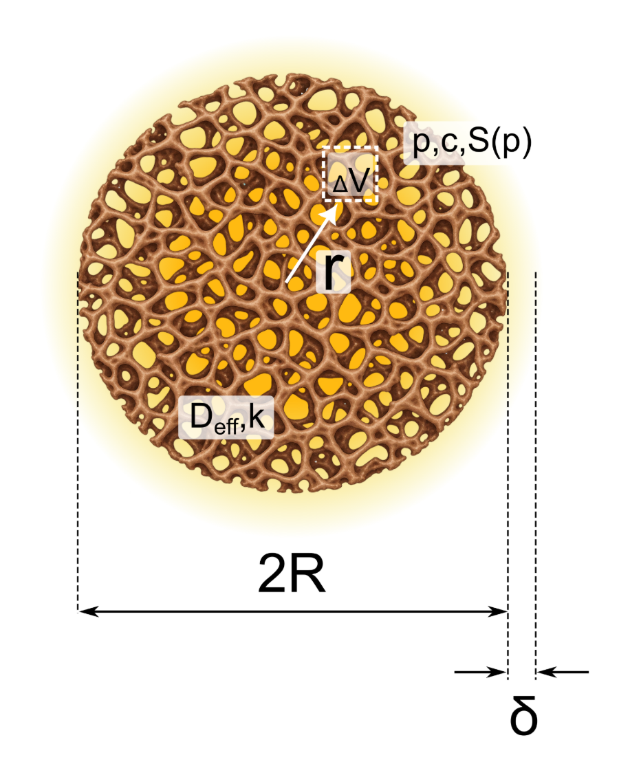
FIG. 1 · EFFECTIVE MEDIUM

Effective-medium representation of a spherical porous silicon particle

Particle of radius R; r points to a representative volume ΔV holding p, c and S(p). Yellow shading is the silicic-acid gradient, the dashed outline the external layer δ.

Nobody has measured the accessible internal area while a particle dissolves. So the area is split into a constant scale S₀ and a dimensionless morphology function σ(p) — the only place where residual geometry enters the model.

(12)

Every candidate satisfies σ(0) = 0; what separates them is the behaviour as p → 1, when the last silicon disappears. Pick a morphology:

σ(p), NORMALISED TO PEAK Fig. 2a, redrawn live

1.00.750.500.250

0 0.25 0.5 0.75 1

porosity, p

read all five at p ={{ th.pText }}

RESIDUAL GEOMETRY · {{ th.selShort }}

peak at {{ th.selPeak }}
as p → 1: {{ th.selAsym }}
σ at p = {{ th.pText }}: {{ th.selVal }}

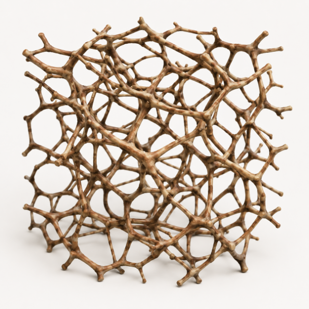
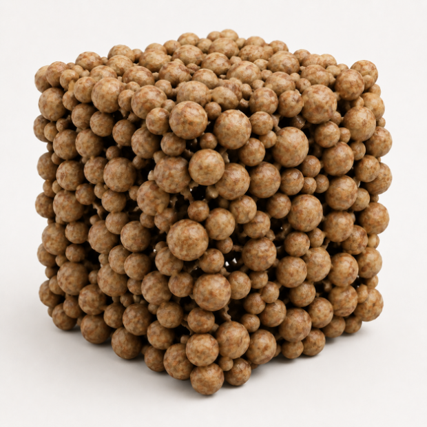
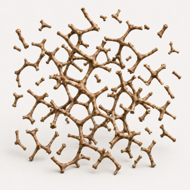
The five functions were chosen to keep a direct physical reading and to stay analytically tractable in both limiting regimes — which is what makes nonlinear fitting of real curves possible at all. Models #1–#3 describe walls, wires and dots; #4 and #5 describe loss of whole residual fragments. In the datasets collected here the fragmentation-type functions fit best, suggesting that fragmentation contributes to the late stages of dissolution.

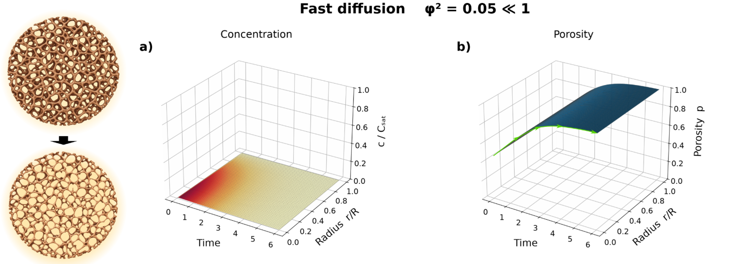
When internal diffusion is fast (φ² << 1), silicic acid leaves the pore network as soon as it forms. Concentration and porosity gradients inside the particle are negligible: the skeleton thins everywhere at once while the outer dimensions barely change.

Numerical solution in the fast-diffusion limit — FIG. 3A–B φ² = 0.05. Concentration stays low everywhere (a) and porosity rises uniformly with radius (b, green arrow) — the particle keeps its size and loses its skeleton from within.

With c ≈ 0 the coupled system collapses to a single ordinary differential equation in the porosity, with one lumped rate constant:

(14)

K has units of inverse time and is the quantity actually fitted to experimental curves throughout this site. Model #2 (nanowires, σ = √(p(1−p))) gives the cleanest illustration: the substitution u = √((1−p)/p) turns the equation into du/dt = −K/2, so

(15)

The solution depends only on p₀, K and t — no numerical integration, no auxiliary inversion — so it can be fitted by ordinary least squares, and F = 0 for t ≥ τ_full. Because p₀ and K are correlated during fitting, measuring the initial porosity independently and fixing it makes K far more reliable. That is exactly why the fitting section asks for porosity first.

The other four

Model #3 (nanodots) is also elementary. Models #1 and #4 need the standard Lambert W function, and Model #5 gives an exact implicit relation — all four remain usable for nonlinear fitting, which is how this site evaluates all five in parallel.

A structural difference matters when you read a long tail in your own data: Models #1–#3 reach complete dissolution in finite time, whereas #4 and #5 produce exponential terminal tails, because σ(p) ∝ 1−p as p → 1. For the fragmentation models the practical figure of merit is therefore t₉₉, not “complete dissolution”.

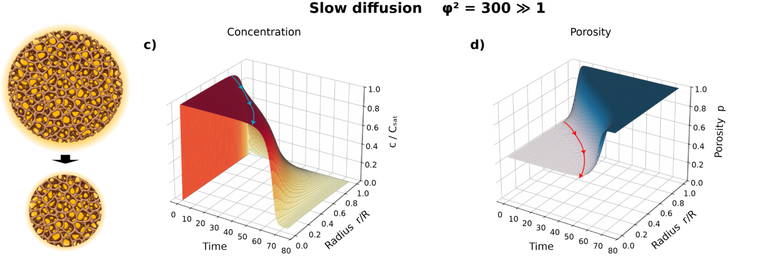
When φ² >> 1 the interior saturates: c → p, the driving force (p − c) vanishes inside, and dissolution survives only in a narrow front that moves inward. The particle is then an undissolved porous core of radius R_f(t) inside an already dissolved shell — a diffusion-controlled shrinking core, except that transport happens through the liquid left behind rather than through a solid product layer.

Numerical solution in the slow-diffusion limit — FIG. 3C–D φ² = 300. The interior sits at saturation (c, blue arrow) and the porosity step travels inward (d, red arrow): the core shrinks while the outer shell is already empty.

Quasi-steady profile in the dissolved shell

In the shell R_f < r < R no solid silicon remains, so the source term is zero. The profile relaxes much faster than the front moves, giving steady spherical diffusion with saturation at the front and a perfect sink at the outer surface:

The gradient of that profile at the front fixes how fast dissolved silicon is carried away:

Front motion

Each mole leaving the front is a mole of solid silicon removed. With ρ_Si(1−p₀) moles of solid per unit volume of the original material, conservation at the moving boundary gives (16); integrating in the relative front position x = R_f/R from x = 1 at t = 0 yields the cubic trajectory and the complete dissolution time:

(16)

(17)

The remaining silicon is just the undissolved core, F = x³. Solving the cubic for the root that falls continuously from 1 to 0 gives the closed form used for fitting, with F = 0 for t ≥ τ_full:

(18)

Note what is missing: σ(p) does not appear. In the strict slow-diffusion limit dissolution is localised at the boundary instead of distributed through the pore volume, so morphology drops out and a single parameter τ_full carries everything. This is also why the design calculator refuses to stretch the slow-limit time by the surface factors f_T, f_pH, f_PEG or f_S — they change the surface rate and the regime criterion, not the diffusion solution.

Planar layer

The same argument in one dimension is simpler still: a linear profile across the dissolved depth s(t), flux D₀C_sat/s, and a square-root front law. For a layer attacked from both sides, L is half the total thickness.

(19)

05 / Cooking Pot

model estimates for material design — require experimental verification

Design a particle, read off its degradation profile

Set the material and the medium in physical terms. The rate coefficient, the transport regime and the curve follow from the chapter’s model — open Calculation details to see every intermediate value.

Particle

Initial porosity {{ cook.fields.p0.unit }}

Specific surface area {{ cook.fields.ssa.unit }}

Surface state · j₀

Source: {{ cook.presetSrc }}

Initial specific flux j₀ {{ cook.fields.j0.unit }}

Taken as already describing your surface at reference conditions — no f_S is applied on top.

Medium

reference: 37 °C, pH 7.4, no PEG

Medium temperature {{ cook.fields.T.unit }}

pH {{ cook.fields.pH.unit }}

PEG coating

PEG molecular weight {{ cook.fields.pegMW.unit }}

Model

φ₀² (regime criterion) {{ cook.phi2 }}

10⁻⁶0.11010⁶

Particle diameter {{ cook.fields.diameter.unit }}

Diffusion slow-down {{ cook.fields.fD.unit }}

Diameter and the slow-down factor enter only φ₀² and the diffusion time — e.g. embedding in a hydrogel. They do not change the surface rate.

Target degradation time

Remaining Si at target, F_Si: {{ cook.targetRemain }}

remaining silicon, F_Si

100%7550250

current design

Applied multipliers

Saved curves

Saved curves share the time axis with the current design, so differences stay visible.

Evidence & extrapolation

•{{ w.t }}

D, m²/s c_s, mol/m³

λ₀ = j₀,app · SSA · M_Si K = λ₀(1−p₀) / (p₀σ(p₀)) φ₀² = j₀,app · SSA · ρ_sk · R² / (D c_s)

In the strict slow limit the diffusion time follows from D, c_s and R only — f_T, f_pH, f_PEG and f_S change the surface rate and the regime criterion, not the diffusion solution.

Watch how your nanoparticle
degrades

Dissolution and diffusion in an evolving porous skeleton

The representative volume

Transport and dissolution

Two geometries

The world outside the particle

Which regime are you in?

The other four

Quasi-steady profile in the dissolved shell

Front motion

Planar layer

Literature degradation datasets

{{ live.title }}

{{ detail.title }}

Fit your own degradation curves

Design a particle, read off its degradation profile

Who made this, and what it builds on

Watch how your nanoparticledegrades

Dissolution and diffusion in an evolving porous skeleton

The representative volume

Transport and dissolution

Two geometries

The world outside the particle

Which regime are you in?

The other four

Quasi-steady profile in the dissolved shell

Front motion

Planar layer

Literature degradation datasets

{{ live.title }}

{{ detail.title }}

Fit your own degradation curves

Design a particle, read off its degradation profile

Who made this, and what it builds on

Watch how your nanoparticle
degrades